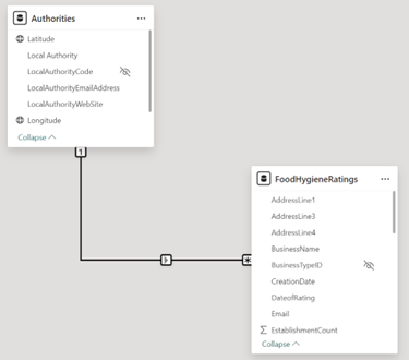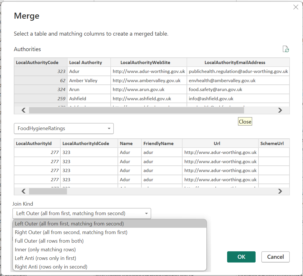
In our final article about data model structures, we will delve deeper into the concept of Joins that we introduced last week. Last week, we became familiar with the importance of relationships, which are crucial for a Semantic Model to work as they connect your fact and dimension tables. In Power BI, there are two main types of Joins that need to be understood: Relationships and Merging. Relationships join modelled or curated tables together for analysis, while Merging is used during the modelling process as part of the Extract, Transform, and Load (ETL) cycle. At each point, different options are available, and they are used for different reasons.
To visualize data in Power BI, we use relationships to simplify the process of determining the required aggregation for evaluation. Each visual in Power BI corresponds to a “Pivot Table” data structure. In this structure, the Dimensions act as the source of Column and Row Headings, while the Fact table provides the aggregations such as SUM(), AVERAGE(), and MAX(). Relationships are utilized to “Filter” the Fact table so that the columns can be evaluated.
It’s important to understand that this concept is fundamental to the Power BI Platform and plays a significant role in addressing the context challenges within it.
In this context, relationships can have three types of joins: one-to-one, one-to-many, and many-to-many, which is also referred to as Cardinality.

One-to-One
These are often considered wasteful within Power BI as the table for both still needs to be evaluated but the granularity for each makes them inefficient. An ideal use case is if you have a Direct Query table with all the extended information and want to import the core elements to facilitate better analysis at the aggregation level, but if the detail is needed, the slower response time is acceptable. Our NYC Bike Data, for example, is being held within a DirectQuery Table; we could decide to bring a subset of that data into the model as an import and then link back to the more detailed table of data via a One-to-One join.
One-to-Many
In Power BI, the One-to-Many and Many-to-One relationships are essentially two sides of the same coin, representing the most frequently encountered relationship types in data modelling. These relationships are characterized by a single, unique value in the Dimension table that correlates to multiple instances in the Fact table. For example, a single customer in the Dimension table may be linked to numerous orders in the Fact table, illustrating the multiplicity of transactions a single entity can generate.
Many-to-Many
In Power BI, Many-to-Many relationships are not directly supported due to their inherent ambiguity. To utilise such relationships effectively, one must establish a directional One-to-Many relationship. This scenario is common between two dimensions and is traditionally resolved by introducing a ‘link table’ to serve as the intermediary fact table. For instance, consider a school timetable involving Students and Teachers; a ‘Classes’ link table can be utilized to associate Students and Teachers with specific Rooms and time periods, thereby simplifying the Many-to-Many relationship into manageable One-to-Many relationships.
When tables are merged within the PowerQuery editor, these merges are a key step in processing data for analysis rather than the actual analysis; however, this does nothing to diminish their importance. The function of these joins are more about shaping the data. Merge joins are the more traditional Join types that are available within Databases.
As these are encountered only during merge actions the source table is always considered the left table, additionally this is expressed as a table within a column. The result is that merge joins can be difficult to fully appreciate.
· Left Outer – Match rows from source with values and return null if no value exists
· Right Outer – Match rows from source and add empty rows to source where no match exists. Additionally drop rows from source that do not have a match.
· Full Outer – Do both Left and Right Outer, so added null rows and null values
· Inner – retain rows ONLY where a match exists
· Left Anti – Keep rows that exist in Source only
· Right Anti – Keep rows that exist on other side only

This is a whistle stop tour of joins within Power BI, the best thing you can do is make sure you are aware that they exist and how best to access them. In database terms joins and relationships are used almost interchangeably and in many circumstances they are the same, however, as with so many things Microsoft related in the context of Power BI they are very different.
Geordie Consulting is a business intelligence and analytics company that helps clients across multiple sectors leverage their data and gain insights. It offers services such as data warehousing, data integration, data visualisation, dashboard development, reporting, and predictive analytics. We have a team of experienced and certified consultants who use the latest tools and technologies to deliver solutions that meet the client’s needs and expectations. Geordie Consulting is your trusted partner for help achieving your goals and objectives through data-driven decisions.