After looking at some generic modelling components it is time to consider the way that measures are held within Power BI, your progression through creating DAX statements and then how best to use them in your whole Data Strategy.
Power BI Measures begin with straightforward auto-sums that are generated by moving columns onto the report canvas. This introductory step encourages users to compose their own custom measures, ultimately guiding them towards employing Field Parameters and Calculation Groups.
Even the most experienced Power BI Developers rely on this fundamental method for generating insights. The initial assessment of a data model’s adequacy often involves combining figures to check its general accuracy, saving time compared to writing out full measures. You have control over this feature by setting the default aggregation type through the “Summarization” settings in the “Column Tools” when you pick a column from the Data panel. With these summarisations, various straightforward reports can be created, which many companies depend on during the early stages of implementing Power BI.
The first measures that people start to write are the ones that emulate Excel, a simple “spreadsheet” style evaluation.
Total = SUM ( [Column] )
These measures expand your capabilities beyond drag-and-drop functionality but do not drastically widen your range of choices. Using these basic measures enables you to accomplish a broader array of reporting tasks and generate numerous insightful reports, yet there may still be restrictions. For more comprehensive context and comparisons, advancing to a more sophisticated level of measure writing might be necessary.
From Simple Measures, you start to write proper measures using more advanced methods.
CALCULATE ( expression, filters )
CALCULATE ( ) inevitably leads to the complexity of Variables. As you get comfortable with variables and computations, you’ll undoubtedly explore the subsequent challenges—calculation Groups and Field Parameters. A common query arises about whether to use one over the other, as if they were mutually exclusive. In truth, each provides distinct functionalities.
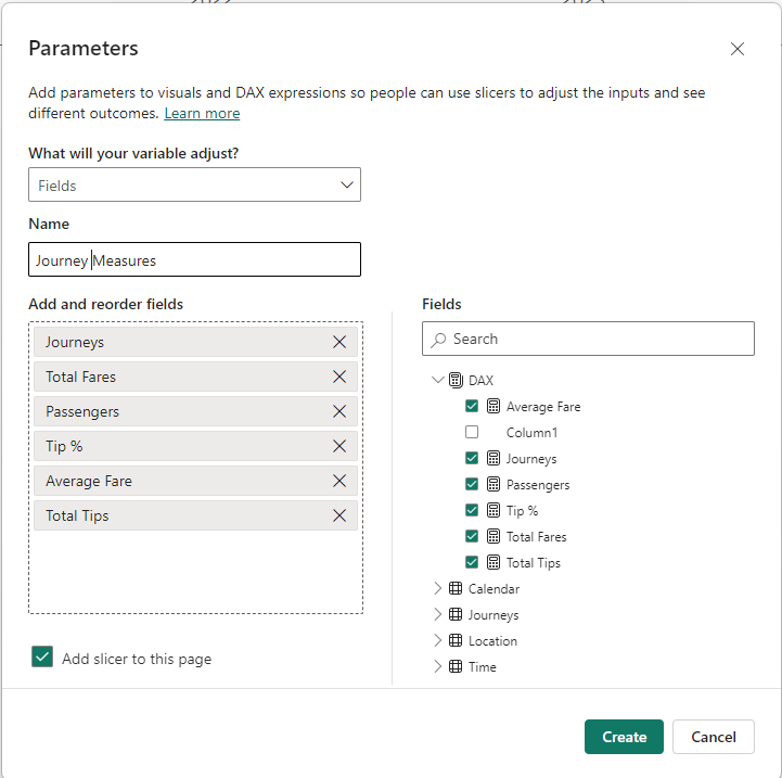
Field Parameters can be defined based on column type or Measures; in this article, we will only look at those that use Measures.
Field Parameters allow you to build a selection of measures that can then be used by your report audience to change the measure that is shown within the visual.


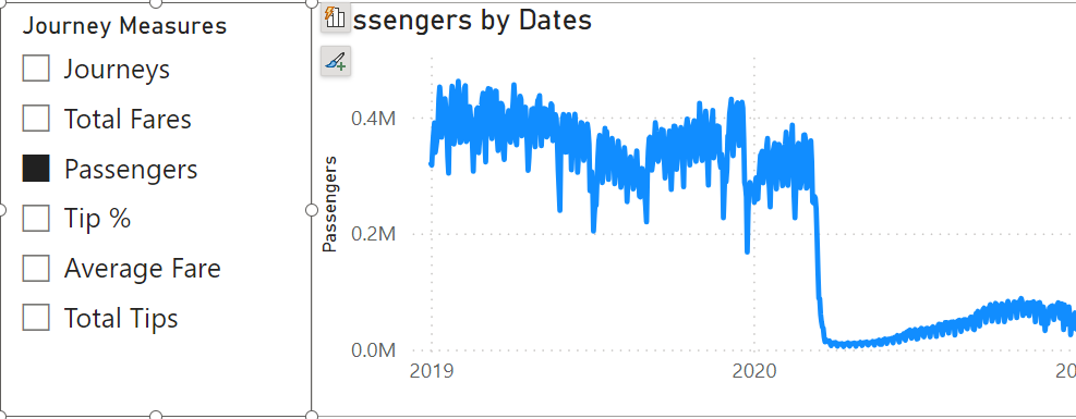
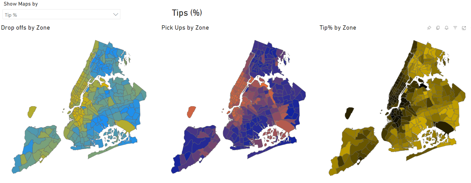
In our example, we have selected to see “Total Passengers” and are looking at them daily. As always, within Power BI, these are evaluated based on the context that they are used — date or location, for example. So, field parameters offer an excellent method to allow an audience to explore a report quickly and efficiently, as a single report page can suddenly be used instead of one page for each measure. One significant benefit of field parameters is that they retain the correct number formatting of their source measure. So, financial measures can be placed with percentages or raw counts (NOTE: that may lead to some interesting issues if you try to show them all together on a single axis).
Field Parameters are a significant benefit when an Organisation uses many core measures as they are relatively user-friendly. In our example, with the Yellow Taxi data, we have Journey (count), Total Fares, Total Tips, Tip %, and Average Fares, all available to be used as needed and just by changing a slicer.

Calculation Groups modify the context of a single measure, making them ideal for scenarios where that measure is repeatedly applied in various contexts, such as with Time Intelligence. Take for instance metrics like Total Sales, Sales MTD (Month-to-Date), Sales QTD (Quarter-to-Date), and Sales YTD (Year-to-Date), along with their preceding period counterparts. Typically, these measures follow a uniform mechanism, so replicating them for additional measures like Profit, Count of Sales, and Refunds quickly becomes labor-intensive. The most efficient approach is to employ Calculation Groups, which function by recalibrating how the current measure displays values based on the Calculation Group.
Current = SELECTEDMEASURE ()
MTD = CALCULATE ( SELECTEDMEASURE(), DATESMTD ( Calendar[Dates] ) )
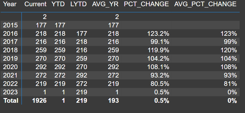
The SELECTEDMEASURE ( ) function represents the measures used with the visual; in practice, Calculation Groups are more often used as “Column” values, as in the table below.
Each Calculation Item within the calculation group can have its own number format, so percentage calculations can be included. DAX measures normally allow you to call a measure within them, it is not recommended to compare other calculation items. This means that the
PCT_CHANGE =
VAR _LY =
CALCULATE (
SELECTEDMEASURE (),
SAMEPERIODLASTYEAR ( DATESYTD ( 'Calendar'[Dates] ) )
)
VAR _YTDCal =
CALCULATE ( SELECTEDMEASURE (), DATESYTD ( 'Calendar'[Dates]) )
VAR _results = DIVIDE ( _YTDCal, _LY )
RETURN
_results
Both the main variables (_LY and _YTDCal) are also Calculation Items within the Calculation Group.

In practice Field Parameters and Calculation Groups work extremely well in tandem as The Field Parameters can be used to define the measure that should be used, while the Calculation Items from the Calculation Group can then be used to enhance their content to produce a whole range of content expanding on the content from the core Field Parameter. If required multiple Calculation Groups can be used.
Geordie Consulting is a business intelligence and analytics company that helps clients across multiple sectors leverage their data and gain insights. It offers services such as data warehousing, data integration, data visualisation, dashboard development, reporting, and predictive analytics. We have a team of experienced and certified consultants who use the latest tools and technologies to deliver solutions that meet the client’s needs and expectations. Geordie Consulting is your trusted partner for help achieving your goals and objectives through data-driven decisions.